Overview
The challenge was to learn and develop a model that could predict optimal inventory levels
Background
My interest in AI grew rapidly after the release of ChatGPT, which reshaped how I thought about automation and problem solving. At the same time, I was increasingly frustrated with manual inventory calculations and forecasts that were often based on intuition or historical averages. Better yet, I thought about how AI could automate and improve these processes. This led to an opportunity to develop an AI inventory forecasting model.
Throughout this guide, I'll walk through my approach, design decisions, and lessons learned. While the implementation isn't shown one-to-one due to data privacy, I'll share the methodology, workflow, and progress so you can see how a similar approach could be applied in your own work!
The Problem
Prior to implementing predictive forecasting, inventory planning relied on historical trends and manual planning processes rather than projected demand signals, leaving decisions highly sensitive to seasonality and external demand fluctuations. This resulted in:
- •Overstocking slow-moving items (Reduced Inventory Agility)
- •Understocking high-demand products (Lost Sales)
- •Inefficient capital allocation
- •Planning was time consuming (Optimize Efficiency)
The Solution
Built a machine learning pipeline that:
- Merged all data sources into a unified dataset
- Engineered features to improve predictive accuracy
- Trained 3 regression models and evaluated performance on historical data
- Generated actionable inventory forecasts with confidence scores
- Automated repetitive calculations to save time and improve decision making
Data Processing Pipeline
Transforming raw data into a unified, ML-ready dataset.
Data Ingestion
Extracted sales, purchase, and inventory data
Data Cleaning
Removed irrelevant columns, handled missing values, standardized SKU formats, and removed duplicates to ensure high-quality data for modeling
Aggregation & Merging
Grouped by SKU to create unified master dataset with all features aligned
Feature Engineering
Created derived metrics to improve model performance
Train/Test Split
Splits to evaluate model performance on unseen data and prevent overfitting
Model Training
Tuning hyperparameters and training regression models to optimize performance
Business Validation
Comparing AI predictions to actual sales and inventory outcomes to ensure forecasts are actionable and reliable
Data Cleaning & Preparation
Arguably the most important step: ensuring high-quality data for model training
Why Data Cleaning Matters
The first step is cleaning the data. Data cleaning is often the most time-consuming yet critical phase of any machine learning project. Raw business data is not perfect, it could contain inconsistencies, missing values, duplicates, and errors that can severely impact model performance.
Without Proper Cleaning
- ✗Poor predictions - garbage in, garbage out
- ✗Model bias - from faulty or missing data
- ✗Training failures - NaN errors or inconsistencies can break algorithms
- ✗Unreliable decisions
With Proper Cleaning
- Accurate predictions - from high-quality training data
- Consistency - forecast accuracy across all SKUs
- Smooth training - proper data prevents crashes
- Trustworthy predictions for decision making
Data Cleaning Steps For Sales
These were the steps taken to clean the sales data before training the model.
Removed Irrelevant Columns
Dropped columns like customer names, product titles, etc. anything that don't contribute to the prediction on optimal order quantity.
cols_to_drop = ['Customer_Name', 'Product_Title', 'Status', 'order_frequency']master_data = master_data.drop(columns=[c for c in cols_to_drop if c in master_data])master_data.head()Missing Values
Checked where data was missing and filled gaps: numeric columns got median values, and purchase quantities were set to zero when no recent orders existed. This way, the dataset stayed complete without breaking the model.
numeric_cols = master_data.select_dtypes(include=['number']).columnsnumeric_cols = [c for c in numeric_cols if "ID" not in c]master_data[numeric_cols] = master_data[numeric_cols].fillna(master_data[numeric_cols].median())master_data[numeric_cols].isnull().sum()Standardized SKU Identifiers
Ensured consistent SKU formatting across all datasets (removed whitespace, converted to uppercase) to enable accurate joins and prevent mismatches.
master_data['SKU'] = master_data['SKU'].str.strip().str.upper()# Identify SKUs in sales missing from datasetorphaned = set(sales_data['SKU'].unique()) - set(master_data['SKU'].unique())Removed Duplicates & Outliers
Identified and removed duplicate SKU records.
master_data = master_data[(master_data['Unit_Price'] > 0) & (master_data['Sales_Quantity'] >= 0)]# Remove duplicate product recordsmaster_data = master_data.drop_duplicates(subset=['SKU'], keep='first')print(f"Data cleaned. Records remaining: {len(master_data)}")Validated Data Types
Converted all numeric fields to appropriate dtypes (int64, float64) and ensured date columns used datetime format. Used errors='coerce' to handle any non-numeric or invalid values, converting them to NaN so they could be filled or handled later. This prevented type errors during model training.
master_data['Sales_Quantity'] = pd.to_numeric(master_data['Sales_Quantity'], errors='coerce')master_data['Unit_Price'] = pd.to_numeric(master_data['Unit_Price'], errors='coerce')# Convert date strings to datetime objectsmaster_data['Order_Date'] = pd.to_datetime(master_data['Order_Date'])print(master_data[['Sales_Quantity', 'Order_Date']].dtypes)Note:
Data cleaning varies across datasets, but the key is to understand your data, identify issues, and filter content to ensure high-quality input for your models. In our model, data was carefully cleaned to achieve accurate inventory forecasts and reliable model performance.
Feature Correlation Analysis
Identifying which features are most strongly correlated with optimal order quantity before training models.
Why Correlation Analysis?
Before training any model, it's important to understand how features relate to each other and to the target variable. Correlation analysis reveals which features have the strongest predictive signal, and identifies redundant features.
Features Analyzed
This was based on a small sample from an example datasetKey Findings
Features with strong correlation are indications to keep an eye on during model training.
Features like Purchase_To_Sales_Ratio showed very low correlation with the target. While not predictive on their own, they were retained for tree-based models that can capture more complex relationships.
Some feature pairs (Sales_Quantity & Total_Demand, Num_Transactions & Total_Transaction_Count) were highly correlated with each other, which is expected since engineered features were derived from raw columns.
Correlation Heatmap
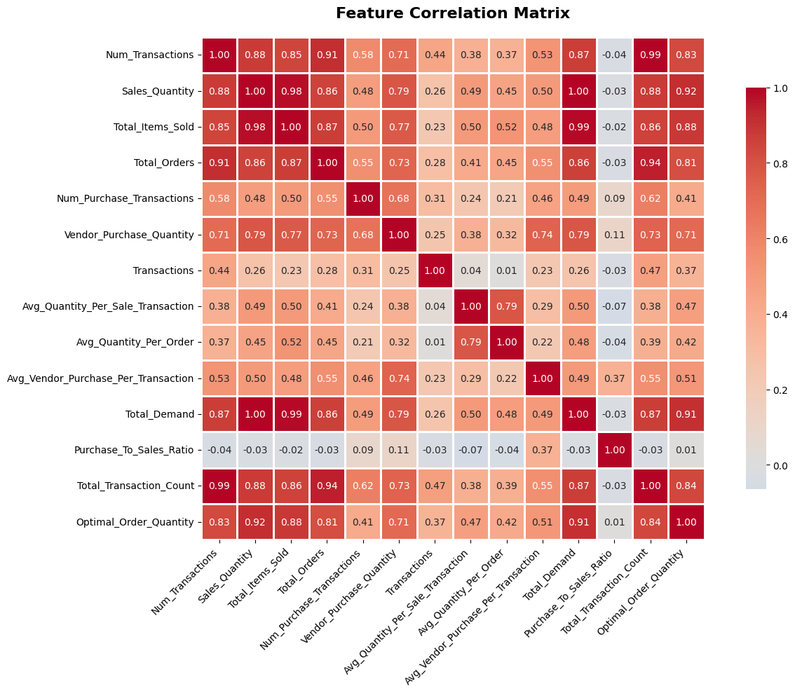
The heatmap of example features
Model Selection & Training
Compared three regression algorithms to find the best predictor of inventory forecasting
Why These Three Models?
I tested three regression models ranging from a basic linear model to advanced methods to see how much complexity the inventory data actually needed, and to make sure more complex models actually improved accuracy.
1. Linear Regression
Linear Regression a base line model that assumes a straight-line relationship between features and the target. It trains instantly, produces interpretable coefficients (showing exactly how much each feature influences the prediction), and answers the question: "Are the relationships in this data fundamentally linear?"
This model was used for the purpose of showing that the data has non-linear relationships. It acheive an R² of 0.68 lowest among the three models, but it was a good starting point to understand the data and set a baseline for improvement with more complex models.
2. Random Forest
Random Forest builds 100 independent decision trees, each trained on a random bootstrap sample of the data with a random subset of features. The final prediction is the average across all trees. This approach was chosen because:
- It captures non-linear relationships and feature interactions that Linear Regression misses
- Bootstrap aggregation (bagging) reduces variance and overfitting
- Provides built-in feature importance scores to understand what drives predictions
- Handling Categorical SKU Data: Great for datasets with categorical features like SKUs, product categories, product types, variants, as it can capture complex patterns without needing extensive preprocessing.
Hyperparameters were set to max_depth=10 to prevent overfitting while still capturing complexity, and min_samples_split=5, min_samples_leaf=2 to ensure each leaf has enough data points for reliable predictions.
3. Gradient Boosting
Unlike Random Forest's parallel approach, Gradient Boosting builds trees sequentially each new tree specifically targets the errors left by the previous one. The mistake strategy was chosen for better accuracy on complex datasets. Gradient Boosting can capture subtle patterns and interactions by refining predictions, which was valuable for inventory data.
- Regularization: L1/L2 penalties allows for more efficient models that generalize better to unseen data
- The learning rate (
0.1) controls how aggressively each tree corrects errors - Shallower trees (
max_depth=5) are used since boosting relies on many weak learners
I wanted to compare whether Gradient Boosting or Random Forest better suits inventory data.
Model Selection Strategy
The three models form a deliberate progression: Linear Regression tests if the problem is linearly solvable, Random Forest explores non-linear patterns with built-in regularization, and Gradient Boosting applies iterative refinement. By comparing all three on the same 80/20 train-test split with StandardScaler normalization, we can directly attribute performance differences to the algorithm choices.
Linear Regression
Baseline Model - R² = 0.68
This model captures some linear relationships but misses the complex patterns in the data, which is reflected in its lower performance compared to the other models. However, it provides valuable insights into which features have a direct linear influence on optimal order quantity through its coefficients.
from sklearn.linear_model import LinearRegression
from sklearn.metrics import r2_score, mean_absolute_error

# Linear Regression - Baseline Model
lr_model = LinearRegression()
lr_model.fit(X_train_scaled, y_train)
lr_predictions = lr_model.predict(X_test_scaled)

# Evaluate Performance
lr_r2 = r2_score(y_test, lr_predictions)
lr_mae = mean_absolute_error(y_test, lr_predictions)

print(f"Linear Regression R²: {lr_r2:.4f}")
print(f"Linear Regression MAE: {lr_mae:.2f}")
Model Comparison Results
Model Comparison & Prediction Analysis
Evaluating and comparing each model's predictive performance using MAE and RMSE to determine the best approach for inventory demand forecasting.
Why MAE & RMSE?
To objectively compare model performance, two key regression metrics were used: Mean Absolute Error (MAE) and Root Mean Squared Error (RMSE). MAE gives the average magnitude of prediction errors in the same units as the target variable, making it easy to interpret. RMSE penalizes larger errors more heavily due to squaring, which is useful for detecting models that occasionally produce significant outlier predictions.
Average of the absolute differences between predicted and actual values. Lower is better. Robust to outliers.
Square root of the average squared differences. Lower is better. Penalizes large errors more than MAE.
Model Results
| Model | R² Score | MAE | RMSE | Verdict |
|---|---|---|---|---|
| Linear Regression | 0.6800 | 24.31 | 32.78 | Baseline |
| Gradient Boosting | 0.8765 | 16.52 | 21.14 | Strong |
| Random Forest | 0.8947 | 14.23 | 18.67 | Best |
Random Forest achieved the lowest MAE (14.23) and RMSE (18.67), meaning its predictions deviate least from actual demand on average and it produces fewer large errors compared to the other models.
Important To Note
Tuning & Hyperparameters
The models shown here use basic hyperparameters as a starting point. In real applications, tuning these parameters can lead to significant performance improvements.
More advanced tuning using GridSearchCV or RandomizedSearchCV could further optimize performance by finding the ideal combination of hyperparameters for your specific dataset. Parameters like min_samples_split, min_samples_leaf, and regularization strength can significantly impact model accuracy and generalization.
Other Variables to Consider
While this model uses transactional and purchase data, real-world inventory forecasting can benefit from incorporating external variables that influence demand patterns:
- •Seasonality & Trends:holidays, drilling season, promotional events
- •Economic Indicators: Commodity prices, inflation rates,
- •Customer Behavior: Order frequency patterns, customer segments, geographic demand shifts
- •Supply Chain Factors: Lead times, supplier reliability, shipping delays
Adding these variables as features could improve predictive power, especially for products with strong seasonal or external dependencies.
Just The Baseline
While achieving 89.5% R² is a strong start, machine learning models require continuous refinement and monitoring to maintain accuracy over time. Business conditions change, customer preferences shift, and new products are introduced all of which can impact model performance.
Next steps for improvement:
- →Monitor model drift and retrain with fresh data quarterly or when performance degrades
- →Experiment with ensemble methods or stacking multiple models for better predictions
- →Build automated pipelines for continuous data ingestion and model retraining
- →Develop confidence intervals or prediction ranges for risk aware decision making
Think of this model as the foundation, not the finished product. Continuous iteration is what turns a good model into a truly reliable business tool.
Prediction Analysis
code.py# Create priority categories based on sales volume and prediction confidence
results_df['Priority'] = 'Medium'
# High priority: High sales volume items
high_sales_threshold = results_df['Sales_Quantity'].quantile(0.75)
results_df.loc[results_df['Sales_Quantity'] >= high_sales_threshold, 'Priority'] = 'High'
# Low priority: Low sales volume items
low_sales_threshold = results_df['Sales_Quantity'].quantile(0.25)
results_df.loc[results_df['Sales_Quantity'] <= low_sales_threshold, 'Priority'] = 'Low'
# Add recommendation categories
results_df['Recommendation'] = 'Maintain'
# Reorder if predicted quantity is significantly higher than current
results_df.loc[results_df['Predicted_Order_Quantity'] > results_df['Purchase_Quantity_2024'] * 1.2, 'Recommendation'] = 'Increase Order'
# Reduce if predicted quantity is significantly lower
results_df.loc[results_df['Predicted_Order_Quantity'] < results_df['Purchase_Quantity_2024'] * 0.8, 'Recommendation'] = 'Decrease Order'
# New items (no 2024 purchase history) - mark for review
results_df.loc[results_df['Purchase_Quantity_2024'] == 0, 'Recommendation'] = 'New Item - Review'
# Sort by priority and sales
results_df_sorted = results_df.sort_values(['Priority', 'Sales_Quantity'], ascending=[True, False])
print("="*100)
print("INVENTORY RECOMMENDATIONS (High Priority Items)")
print("="*100)
for priority in ['High', 'Medium', 'Low']:
priority_df = results_df_sorted[results_df_sorted['Priority'] == priority]
print(f"
{priority} Priority Items: {len(priority_df)}")
print("-" * 100)
print(priority_df.head(5)[['SKU', 'Sales_Quantity', 'Predicted_Order_Quantity',
'Recommendation']].to_string(index=False))
print("
" + "="*100)
print("RECOMMENDATION SUMMARY")
print("="*100)
print(results_df['Recommendation'].value_counts().to_string())
====================================================================================================
INVENTORY RECOMMENDATIONS (High Priority Items)
====================================================================================================

High Priority Items: 75
----------------------------------------------------------------------------------------------------
         SKU   Sales_Quantity  Predicted_Order_Quantity    Recommendation
    Product_1             4794.0                     10219    Decrease Order
    Product_2             2661.0                      5278 New Item - Review
    Product_3             2539.0                      9977          Maintain
    Product_4             2440.0                      9084    Increase Order
    Product_5             1946.0                      5643          Maintain
Cross-Validation Strategy: Time Series Split
I used Time Series Split instead of regular k-fold cross-validation. Since inventory data has a time component, it's important to train on past data and validate on future periods. This prevents the model from "cheating" by looking ahead, which can happen with standard cross-validation.
With time series split, the model learns from progressively larger chunks of historical data and is tested on the next time period. This mimics real-world forecasting, where we're always predicting future demand based on what's already happened.
Why Time Series Split? Standard k-fold shuffles data randomly, which can end up training on “future” data and testing on the “past,” giving results that aren't realistic. A time series split makes sure the model only learns from the past, so the validation scores actually reflect how it would perform in real life.
Business Impact & Recommendations
How this model translates into real operational value and where it can go from here.
The Real Model Behind the Scenes
What you see in this project is a simplified version of inventory forecasting. I was part of a team that had the opportunity to develop a deeper production model that continuously ingests new data and improves over time to increase forecasting accuracy.
Specifically, the production model incorporates signals such as global news events, oil and gas industry updates, and macroeconomic indicators. In industries where commodity pricing and global events directly impact demand, integrating these external data sources allows the model to better anticipate future trends rather than relying solely on historical patterns.
What It Actually Did for Operations
Before this model, a lot of inventory decisions came down to manual spreadsheets and gut feeling. The model changed that. It cut down the time I spent on manual calculations, removed a lot of the guesswork, and acted as a second opinion that I could trust when making purchasing decisions.
Order Timing Optimization
The model's predictions helped timing orders better with indicators and led to more efficient inventory management.
Fewer Stockouts
Demand forecasting flagged items at risk before they ran out, so I could act proactively.
Reduced Overstocking
Less money tied up in excess stock and freed up warehouse space
Confident Decisions
Having data backed recommendations gave me and the team confidence to commit to purchasing decisions.
Future Enhancements & Roadmap
Planned improvements and additional features to enhance the inventory forecasting system.
Short-Term Improvements (Next 3 Months)
Time Series Features
Incorporate temporal patterns (seasonality, trends, day-of-week effects) using lag features and rolling averages.
External Data Integration
Add market trends, competitor pricing, and economic indicators to capture demand drivers beyond internal data.
Hyperparameter Optimization
Use GridSearchCV or Bayesian optimization to fine-tune max_depth, n_estimators, and learning rates systematically.
SKU Segmentation
Train separate models for high/medium/low velocity SKUs to specialize predictions for different demand patterns.